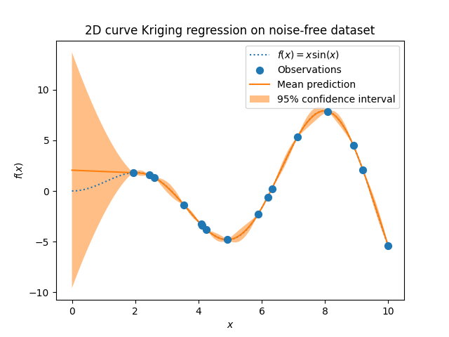
2D curve kriging with confidence estimation

This example shows how to interpolate a 2D curve with confidence estimation.

\[y = f(x)\]

The curve is defined by a set of points \((x_i, y_i)\), where \(i = 1, 2, ..., n\).

This kriging method is the basis for fiber tow trajectory smoothing and control point resampling of fiber tow surface implemented in PolyTex.Tow class.

import numpy as np
from polytex.kriging import curve2D
import polytex as ptx
import matplotlib.pyplot as plt

Make up some data

X = np.linspace(start=0, stop=10, num=300)
y = X * np.sin(X)

# Choose some data points randomly to build the kriging model
rng = np.random.RandomState(1)
training_indices = rng.choice(np.arange(y.size), size=16, replace=False)

X_train, y_train = X[training_indices], y[training_indices]

data_set = np.hstack((X_train.reshape(-1, 1), y_train.reshape(-1, 1)))

Dual kriging formulation

For most users, this part can be ignored. It is only for the purpose of understanding the formulation of dual kriging. In practice, the kriging interpolation can be used by calling the function curve2D.interpolate directly.

# Kriging parameters
name_drift, name_cov = 'lin', 'cub'

# The smoothing factor is used to control the smooth strength of the parametric
# curve. The larger the smoothing factor, the smoother the curve. However, the
# curve may deviate from the data points. For a zero smoothing factor, the curve
# passes through all the data points.
smoothing_factor = 0


mat_krig, mat_krig_inv, vector_ba, expr1, func_drift, func_cov = \
    curve2D.curve_krig_2D(data_set, name_drift, name_cov, nugget_effect=smoothing_factor)

Kriging interpolation

Kriging model and prediction with mean, kriging expression and the corresponding standard deviation as output.

mean_prediction, expr2, std_prediction = curve2D.interpolate(
    data_set, name_drift, name_cov,
    nugget_effect=smoothing_factor, interp=X, return_std=True)

# Plot the results
plt.plot(X, y, label=r"$f(x) = x \sin(x)$", linestyle="dotted")
plt.scatter(X_train, y_train, label="Observations", s=50, zorder=10)
plt.plot(X, mean_prediction, label="Mean prediction")
plt.fill_between(X.ravel(),
                 mean_prediction - 1.96 * std_prediction,
                 mean_prediction + 1.96 * std_prediction,
                 alpha=0.5, label=r"95% confidence interval")

plt.legend()
plt.xlabel("$x$")
plt.ylabel("$f(x)$")
_ = plt.title("2D curve kriging regression on noise-free dataset")

plt.show()

Save the kriging model

You can save the kriging model to a file for later use and load it back using ptx.load() function. Note that the kriging model is saved in a Python dictionary with its name as the key.

expr_dict = {"cross": expr2}
ptx.pk_save("./test_data/FunXY.krig", expr_dict)

# Reload the kriging model
expr_load = ptx.pk_load("./test_data/FunXY.krig")